You will be provided with images scanned by 4 different scanners, 3 out of which are labeled. In total the set consists of 200 cases of breast cancer.
The following text is taken from the challenge report (Aubreville et al., "Mitosis domain generalization in histopathology images — The MIDOG challenge", Medical Image Analysis, 2023, arXiv:2204.03742).
Challenge cohort
The challenge dataset consists of 300 breast cancer cases and was curated from a retrospective, consecutive selection taken from the diagnostic archive of the University Medical Center (UMC) Utrecht, The Netherlands. All samples were resected solely for diagnostic purposes. Inclusion criteria were the availability of the microscopy (glass) slide, a confirmed breast cancer excision (as documented in the patient record), the availability of a pathology report with a documented mitotic count and that the patients did not opt out for the use of their data in research projects. Prior to handing over to project partners within the organization committee, all slides and clinical meta data were anonymized. Additionally, for the use in the challenge we obtained approval by the institutional review board of UMC Utrecht (reference: TCBio 20-776).
The specimen was preprocessed according to clinical standard routine and stained with hematoxylin and eosin (H&E) dye. Subsequently, the cases were randomly split into the training set (200 cases) and the preliminary (20 cases) and final (80 cases) test set. Within each of those sets, we performed another random split, to assign the cases to the scanners, i.e. we split up the 200 cases of the training set into 50 cases for each of the four training scanners (A,B,C,D, see below), and the 80+20 cases of the test sets into 20+5 for each of the the four test scanners (A,D,E,F, see below). By this procedure, we can expect no significant biases in any of the subsets of the dataset and assume a high degree of representativeness.
Image acquisition
We used four different scanners for the digitization of the training set. Scanner A is the scanner that is used in clinical practice to digitize all slides at UMC Utrecht. Therefore, all slides of our dataset are also available scanned by this scanner and we use this as our reference scanner to counter a possible scanner-caused bias in the region of interest selection. For the test set, we used a mix of known and unknown scanners to test simultaneously for performance on in-domain scanners and for generalization to out-of-domain scanners. For scanner D, which was part of the training and the test set, no labels were provided as part of the training set. Hence, this scanner was included for the sole purpose of providing data for approaches performing unsupervised domain adaptation.
Scanners and cases
Table compiled from the scanner descriptions and case numbers given in sections 2.1 and 2.2 of the challenge report.
| Scanner | Model | Resolution | Training set | Preliminary test set | Final test set |
|---|---|---|---|---|---|
| A | Hamamatsu NanoZoomer XR (C12000-22) | 0.23 µm/px (40x) | 50 cases (labeled) | 5 cases | 20 cases |
| B | Hamamatsu NanoZoomer S360 | 0.23 µm/px (40x) | 50 cases (labeled) | – | – |
| C | Aperio Scanscope CS2 (Leica Biosystems) | 0.25 µm/px (40x) | 50 cases (labeled) | – | – |
| D | Leica Aperio GT 450 | 0.26 µm/px (40x) | 50 cases (no labels) | 5 cases | 20 cases |
| E | 3DHISTECH Panoramic 1000 | 0.24 µm/px (20x) | – | 5 cases | 20 cases |
| F | Hamamatsu NanoZoomer 2.0RS (C10730-12) | 0.23 µm/px (40x) | – | 5 cases | 20 cases |

Random crops of breast cancer tissue from all six scanners of the training and test set, showing the visual variability between the scanners. (Figure 2 of the challenge report)
Each of the slides was scanned by the assigned WSI scanner as well as by the clinical reference scanner (Scanner A). To reduce bias which might be caused by different tissue representation on other scanners, a trained pathologist (C.B.) selected a region of interest spanning 2.0 mm² on the reference scans. For streamlined dataset creation, all WSIs were uploaded to a central server running a collaborative annotation software. There, the reference scans were registered to the respective image acquired by different scanners using a quadtree-based WSI registration method by Marzahl et al. The registration was manually fine-tuned and quality checked subsequently. Finally, the defined ROIs were extracted from the images acquired by all scanners. For the Leica and Aperio scanner, the scanners color profile was available from the WSIs, which enabled the organizers to convert those images into the standard RGB color space. Regardless of this step, significant differences in color can be observed (see fig. 3).
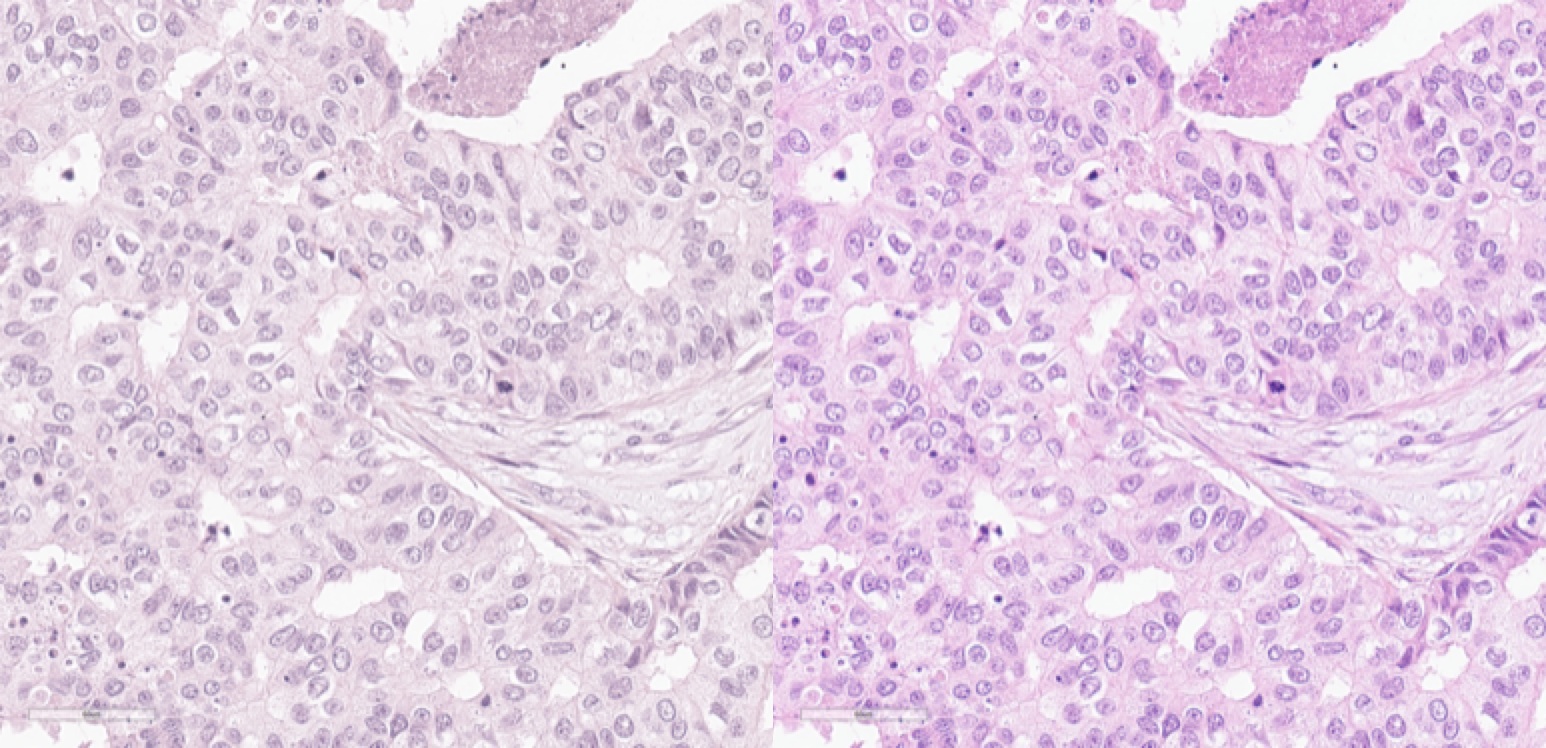
Image from Scanner D in the original (left) scanner color space and in the standard RGB color space (right). (Figure 3 of the challenge report)
Labeling
In the process of labeling, three expert pathologists (C.B., R.K., T.D.) were involved. All experts work at different institutions (in different countries) and have 6+ years of professional experience and a demonstrably high level of expertise in mitotic figure recognition. Additionally, all experts agreed on common criteria for mitotic figure identification.
The inter-rater variability of mitosis identification can be attributed to two main factors: Most notably, experts disagree on individual mitotic figures (object-level disagreement) due to morphological overlap with imposters. For this reason, most mitotic figures datasets were annotated as consensus voting between multiple experts. Additionally, as mitotic figures can be considered sparse events in most WSIs and sometimes faint structures, experts tend to miss especially less recognizable objects when screening the image.
To account for both effects and create a high-quality dataset, we employed a machine learning-aided strategy: Initially, a single experienced expert (C.B.) screened all ROIs for mitotic figures and for a roughly equal number of imposters / hard negatives (non-mitotic cells with morphological similarity to mitotic figures). We trained a customized RetinaNet to identify cells that were missed in this initial labeling (mitotic figure candidates). Using a very low detection threshold on the model output, we ensured that this approach yielded high sensitivity (and low specificity). All mitotic figure candidates were then handed to the primary expert, again, to sort into missed mitotic figures and non-mitotic structures (which comprised the vast majority). To reduce bias in the labeling process introduced by the first expert, all manual cell labels and detections from the algorithmic augmentation step were class-blinded and handed to a secondary expert (R.K.). The secondary expert then sorted all cells into mitotic figures and non-mitotic cells. In the case of agreement, the label was accepted as ground truth. In case of disagreement, the cells were again class-blinded and given to a third expert (T.D.), who then made the final decision.
In the dataset, the challenge organizers provided squared approximated bounding boxes of equal size (50px) to the participants. The non-mitotic cells (hard negatives) were provided alongside the true mitotic figures to enable the use within sampling schemes.
Dataset statistics
As fig. 4 shows, the mitotic count (MC) (i.e., the number of mitoses per 2.0 mm²) follows a similar distribution over all scanners in the original pathology report and the MIDOG dataset. Differences between the MC of the pathology report and the MIDOG dataset were not significant (two-sided paired t-test: p-value: 1.000, scipy stats package version 1.7.3). The intraclass correlation (ICC, two-way, single measurements, random raters) of the MC ratings indicate a substantial agreement (ICC2=0.684, pingouin package version 0.5.1) as of the definition by Hallgren, which can be attributed to different reasons. Firstly, it cannot be guaranteed that the slides that were included in this dataset were the same that were used for clinical MC assessment, as oftentimes multiple slides per case exist. Secondly, the annotation methodology used here differs substantially from how the MC is determined in a clinical setting. Lastly, even if the same slides were used, the MC is known to be highly area-dependent, which might further contribute to the discordance. As depicted in fig. 4, there is a high number of potentially low-grade tumors within the dataset, which is, however, reflective of the general population of cases at a tertiary hospital.
Data usage
All data of the training set was released under the Creative Commons 4.0 BY (attribution) NC-ND (non-commercial, non-derivative) license.
See Getting the data for download information.